机器学习 | Transformer
Transformer:一种采用注意力机制的深度学习模型,这一机制可以按输入数据各部分重要性的不同而分配不同的权重。
上一篇关于注意力机制的笔记实际上已经介绍了 Transformer 中最“灵魂”的注意力模块,这一篇笔记更加注重的是 Transformer 的整体结构,并且方式不再是公式推导而是使用代码实现。
本篇笔记使用 PyTorch 进行代码实现,模型结构参照原论文 Attention Is All You Need. 本篇笔记内容参考了文章 Mastering Transformer: Detailed Insights into Each Block,如果感兴趣可以看一下原作者完整的三篇教程,写得真的很好。
1 总览
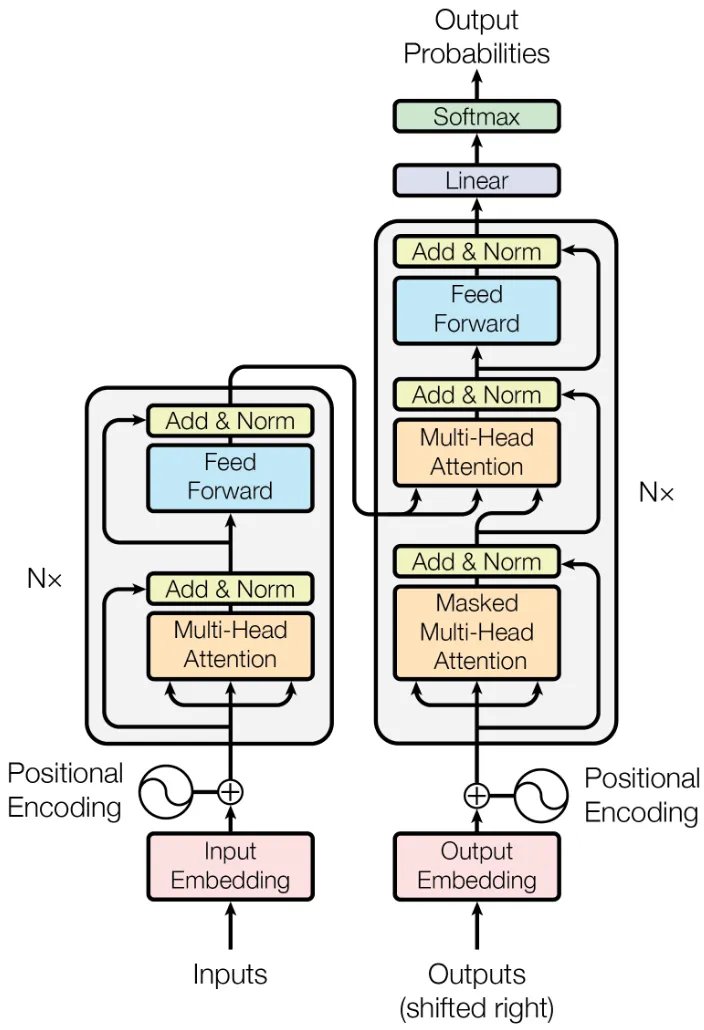
原论文 Attention Is All You Need 中 Transformer 的整体结构的图示如上,归纳一下它包含的模块,也就是我们要一个个实现的内容:
- Embedding:嵌入层,将 Token 嵌入为向量。
- PositionalEncoding:位置编码,给序列添加位置信息。
EncoderBlock:编码器块(原版 Transformer 用的 Encoder-Decoder 架构).
- MultiHeadAttentionBlock:多头自注意力块。
- FeedForwardBlock:前馈神经网络块。
- ResidualConnection:残差连接,对应图中 Add & Norm 的 Add 步骤。
- LayerNorm:层归一化,对应图中 Add & Norm 的 Norm 步骤。
DecoderBlock:解码器块。
- (Masked)MultiHeadAttentionBlock:多头自注意力块。
- MultiHeadAttentionBlock:多头交叉注意力块。
- FeedForwardBlock:前馈神经网络块。
- ResidualConnection:残差连接,对应图中 Add & Norm 的 Add 步骤。
- LayerNorm:层归一化,对应图中 Add & Norm 的 Norm 步骤。
- LinearProjection:线性分类头,用于得到最终预测 Token.
2 Embedding 嵌入层
2.1 原理
嵌入层负责将 Token 嵌入为向量,具体来说就是根据 Token ID,查表得到这个 Token 对应的嵌入向量。
嵌入层有两个变量,分别是代表模型维度的 $d_{\text{model}}$ 与词表大小 $\text{vocabsize}$,嵌入层的参数便是 $d_{\text{model}}\times\text{vocabsize}$ 大小的矩阵 $\boldsymbol{W}_{\text{embed}}$。当要嵌入 ID 为 $x$ 的 Token,那么便抽取矩阵 $\boldsymbol{W}_{\text{embed}}$ 的第 $x$ 列,得到的维度为 $d_{\text{model}}$ 的向量就是 Token 的嵌入向量了。
2.2 实现
代码实现直接使用 PyTorch 的 nn.Embedding 即可。
class Embedding(nn.Module):
    def __init__(self, d_model: int, vocab_size: int):
        super().__init__()
        self.d_model = d_model
        self.d_vocab = vocab_size
        self.embedding = nn.Embedding(vocab_size, d_model)

    def forward(self, x):
        return self.embedding(x) * math.sqrt(self.d_model)
3 PositionalEncoding 位置编码
3.1 原理
论文原文给出的位置编码公式如下:
$$ PE_{(k,2i)}=\sin(k/10000^{2i/d_{\mathrm{model}}})\\ PE_{(k,2i+1)}=\cos(k/10000^{2i/d_{\mathrm{model}}}) $$
举例来说,如果 $d_{\text{model}}=6$,序列长度为 $4$,那么位置编码如下:
| Token | Index | $PE_{(k,0)}$ | $PE_{(k,1)}$ | $PE_{(k,2)}$ | $PE_{(k,3)}$ | $PE_{(k,4)}$ | $PE_{(k,5)}$ |
|---|---|---|---|---|---|---|---|
| What | $k=0$ | $\sin(0/1)=0.000$ | $\cos(0/1)=1.000$ | $\sin(0/21.544)=0.000$ | $\cos(0/21.544)=1.000$ | $\sin(0/464.159)=0.000$ | $\cos(0/464.159)=1.000$ |
| can | $k=1$ | $\sin(1/1)=0.842$ | $\cos(1/1)=0.540$ | $\sin(1/21.544)=0.046$ | $\cos(1/21.544)=0.999$ | $\sin(1/464.159)=0.002$ | $\cos(1/464.159)=1.000$ |
| I | $k=2$ | $\sin(2/1)=0.909$ | $\cos(2/1)=-0.416$ | $\sin(2/21.544)=0.093$ | $\cos(2/21.544)=0.996$ | $\sin(2/464.159)=0.004$ | $\cos(2/464.159)=1.000$ |
| say | $k=3$ | $\sin(3/1)=0.141$ | $\cos(3/1)=-0.990$ | $\sin(3/21.544)=0.139$ | $\cos(3/21.544)=0.990$ | $\sin(3/464.159)=0.007$ | $\cos(3/464.159)=1.000$ |
一行一行观察上表,每一行代表一个 Token 的位置编码。
一列一列观察上表,每一列都相当于对 $\sin$ 或 $\cos$ 函数进行间隔为 $1$ 的采样,从左到右的每一列,三角函数的周期实际上是增大的。
因此,这种正弦位置编码 (Sinusoidal Positional Encoding) 实际上就是通过组合不同频率的三角函数来表示位置。
要理解为什么不同频率的周期函数能表示位置,不妨找一个更简化的相似的例子,即用二进制来表示位置。如果 $d_{\text{model}}=4$,序列长度为 $8$,用二进制表示位置如下(低位在左):
| Token | Index | $PE_{(k,0)}$ | $PE_{(k,1)}$ | $PE_{(k,2)}$ | $PE_{(k,4)}$ |
|---|---|---|---|---|---|
| He | $k=0$ | 0 | 0 | 0 | 0 |
| went | $k=1$ | 1 | 0 | 0 | 0 |
| up | $k=2$ | 0 | 1 | 0 | 0 |
| the | $k=3$ | 1 | 1 | 0 | 0 |
| hill | $k=4$ | 0 | 0 | 1 | 0 |
| with | $k=5$ | 1 | 0 | 1 | 0 |
| his | $k=6$ | 0 | 1 | 1 | 0 |
| friend | $k=7$ | 1 | 1 | 1 | 0 |
将这个二进制的位置编码和上面的正弦位置编码对比,很容易发现相似之处:一列一列来观察,每一列都是不同周期的周期函数,从左到右的每一列,函数的周期是增大的。因此,用二进制来表示位置编码实际上和正弦位置编码的底层原理一致,都是通过组合不同频率的周期函数来表示位置。
3.2 实现
直接按照论文的公式进行朴素实现当然是可行的,但是为了代码实现的更简洁以及向量化,首先对公式进行变形:
$$ \frac{k}{10000^{\frac{2i}{d_{\mathrm{model}}}}}=\frac{k}{e^\frac{2i\ln10000}{d_{\mathrm{model}}}}=k\cdot e^{-\frac{2i\ln10000}{d_{\mathrm{model}}}} $$
变形成乘法形式之后,那么对于 $\sin$ 或 $\cos$ 里的值形成的矩阵,便可以拆分为两个向量相乘了,这样的实现方法效率更高。
$$ \begin{bmatrix} 0\cdot e^{-\frac{0\ln10000}{d_{\mathrm{model}}}} & 0\cdot e^{-\frac{2\ln10000}{d_{\mathrm{model}}}} & \cdots & 0\cdot e^{-\frac{2i\ln10000}{d_{\mathrm{model}}}}\\ 1\cdot e^{-\frac{0\ln10000}{d_{\mathrm{model}}}} & 1\cdot e^{-\frac{2\ln10000}{d_{\mathrm{model}}}} & \cdots & 1\cdot e^{-\frac{2i\ln10000}{d_{\mathrm{model}}}}\\ \vdots & \vdots & \ddots & \vdots\\ m\cdot e^{-\frac{0\ln10000}{d_{\mathrm{model}}}} & m\cdot e^{-\frac{2\ln10000}{d_{\mathrm{model}}}} & \cdots & m\cdot e^{-\frac{2i\ln10000}{d_{\mathrm{model}}}} \end{bmatrix}=\begin{bmatrix} e^{-\frac{0\ln10000}{d_{\mathrm{model}}}} & e^{-\frac{2\ln10000}{d_{\mathrm{model}}}} & \cdots & e^{-\frac{2i\ln10000}{d_{\mathrm{model}}}} \end{bmatrix}\begin{bmatrix} 0\\ 1\\ \vdots\\ m \end{bmatrix} $$
In addition, we apply dropout to the sums of the embeddings and the positional encodings in both the encoder and decoder stacks.
还有需要注意的一点是,论文中指明位置编码处进行了 Dropout,因此实现时也要还原这一点。
class PositionalEncoding(nn.Module):
    def __init__(self, d_model: int, seq_len: int, dropout: float):
        super().__init__()

        self.d_model = d_model
        self.seq_len = seq_len
        self.dropout = nn.Dropout(dropout)

        # idx.shape = (seq_len, 1)
        idx = torch.arange(0, seq_len, dtype=torch.float).unsqueeze(1)
        # div.shape = (d_model // 2, )
        div = torch.exp(torch.arange(0, d_model, 2).float() * (-math.log(10000.0) / d_model))
        # (idx * div).shape = (seq_len, d_model // 2)

        pe = torch.zeros(seq_len, d_model)
        pe[:, 0::2] = torch.sin(idx * div)
        pe[:, 1::2] = torch.cos(idx * div)
        pe.unsqueeze_(0) # shape = (1, seq_len, d_model)

        self.register_buffer('pe', pe)

    def forward(self, x):
        x = x + self.pe[:, :x.size(1)]
        return self.dropout(x)
4 LayerNorm 层归一化
4.1 原理
LayerNorm 的公式如下,即先进行一次归一化,再进行一次仿射变换:
$$ y = \alpha \cdot \frac{x - \mu}{\sigma + \epsilon} + \beta $$
其中 $\epsilon$ 的作用是防止 $\sigma=0$ 时发生除零错误。
4.2 实现
class LayerNorm(nn.Module):
    def __init__(self, dim: int, eps: float = 1e-6):
        super().__init__()
        self.eps = eps
        self.alpha = nn.Parameter(torch.ones(dim))
        self.beta = nn.Parameter(torch.zeros(dim))

    def forward(self, x):
        mean = x.mean(-1, keepdim=True)
        std = x.std(-1, keepdim=True)
        return self.alpha * (x - mean) / (std + self.eps) + self.beta
5 ResidualConnection 残差连接
残差连接的原理已经有往期笔记(残差神经网络)介绍,因此直接开始介绍实现。
We apply dropout [33] to the output of each sub-layer, before it is added to the sub-layer input and normalized.
实现时需要注意论文中说明的,Sub Layer、残差连接、层归一化和 Dropout 的顺序。根据论文描述,顺序应该如下:
$$ \mathrm{LayerNorm}(x + \mathrm{Dropout}(\mathrm{Sublayer}(x))) $$
class ResidualConnection(nn.Module):
    def __init__(self, d_model: int, dropout: float):
        super().__init__()
        self.dropout = nn.Dropout(dropout)
        self.norm = LayerNorm(d_model)

    def forward(self, x, sublayer):
        return self.norm(x + self.dropout(sublayer(x)))
6 FeedForwardBlock 前馈神经网络块
前馈神经网络的原理已经有往期笔记(BP 神经网络)介绍,因此直接开始介绍实现。
class FeedForwardBlock(nn.Module):
    def __init__(self, d_model: int, d_hidden: int, dropout: float):
        super().__init__()
        self.linear_1 = nn.Linear(d_model, d_hidden)
        self.dropout = nn.Dropout(dropout)
        self.linear_2 = nn.Linear(d_hidden, d_model)

    def forward(self, x):
        x = self.linear_1(x)
        x = torch.relu(x)
        x = self.dropout(x)
        x = self.linear_2(x)
        return x
7 MultiHeadAttentionBlock 多头注意力块
注意力机制的原理已经有往期笔记(注意力机制)介绍,因此直接开始介绍实现。
在 Transformer 中,使用的是多头注意力块,其相较于普通的单头注意力更加强大。
参数
首先需要注意多头注意力的参数,一共有四个矩阵:$\boldsymbol{W}_q,\boldsymbol{W}_k,\boldsymbol{W}_v,\boldsymbol{W}_o$,大小均为 $(d_{\text{model}},d_{\text{model}})$.
如果阅读过原论文,应该注意到这四个矩阵的大小应该分别是 $(d_{\text{model}},d_q),(d_{\text{model}},d_k),(d_{\text{model}},d_v),(d_v,d_{\text{model}})$ 而不是我所说的这个方阵。实际上这里将这四个参数都取为方阵只是为了实现的方便,即假定 $d_q=d_k=d_v$.
另外,我的上一篇笔记并不是用的 $\boldsymbol{W}_v,\boldsymbol{W}_o$ 来表示两次线性变化,而是使用的 $\boldsymbol{W}_{v\downarrow},\boldsymbol{W}_{v\uparrow}$. 实际上这只是记法不同,本篇文章使用原论文的记法,即 Q, K, V, O 四个矩阵。上一篇笔记中还提到每个注意力头拥有独立的参数 Q, K, V,实际上在实现中它们仍然储存为一个整体的矩阵,在矩阵运算中自然而然地分给了几个注意力头,而不需要显式地分成多个矩阵。
计算
在实现中,弄清楚矩阵运算每一步的 Tensor 大小至关重要。我们一步一步分析:
def forward(self, X_q, X_k, X_v, mask=None):
    ...
首先传入 $X_q, X_k, X_v$ 三个张量,这三个张量的大小应当都是 $(batch,seq,d_{\text{model}})$,其中 $batch$ 为设定的 batch_size,$seq$ 为 Token 序列长度。
query = self.W_q(X_q)
key = self.W_k(X_k)
value = self.W_v(X_v)
然后通过 $\boldsymbol{W}_q,\boldsymbol{W}_k,\boldsymbol{W}_v$ 三个矩阵进行线性变化,大小仍然是 $(bs,seq,d_{\text{model}})$.
query = query.view(query.shape[0], query.shape[1], self.num_heads, self.d_k).transpose(1, 2)
key = key.view(key.shape[0], key.shape[1], self.num_heads, self.d_k).transpose(1, 2)
value = value.view(value.shape[0], value.shape[1], self.num_heads, self.d_k).transpose(1, 2)
接下来便要切分注意力头,然后将参数分给每个头。
首先就是切分,view 方法做的事情实际上就是将 $d_{\text{model}}$ 大小的维度拆成 $head$ 和 $d_k$ 大小的两个维度,其中 $head$ 为设定的注意力头数,$d_k$ 为每个注意力头的维度。即拆分后张量大小为 $(batch,seq,head,d_k)$.
然后便是将参数分给每个头,经过上面的拆分实际上会发现每个注意力头的参数不连续,通过 transpose 方法调换第 $1,2$ 维就连续了。调换后的张量大小为 $(batch,head,seq,d_k)$.
接下来就是计算注意力的流程了,公式如下:
$$ \text{Attention}(Q, K, V) = \text{softmax}\left(\frac{QK^T}{\sqrt{d_k}}\right)V $$
attn_scores = torch.matmul(Q, K.transpose(-1, -2)) / math.sqrt(self.d_k)$Q,K$ 的大小都是 $(batch,head,seq,d_k)$,要做矩阵乘法得话得转置,$K^T$ 的大小是 $(batch,head,d_k,seq)$. 做完乘法后结果的大小为 $(batch,head,seq,seq)$,即注意力矩阵。还要记得除以 $\sqrt{d_k}$ 这个缩放项,有助于稳定模型。
if mask is not None:
    attn_scores.masked_fill_(mask == 0, -1e9)
然后便是遮罩,给指定位置赋值为 $-\infty$,用 $-10^{9}$ 这个极小数来表示。
attn_probs = attn_scores.softmax(-1)
attn_probs = self.dropout(attn_probs)
然后是列 Softmax,给 softmax 方法的 dim 参数传入 -1 指定方向。做完后进行一次 Dropout. 进行 Softmax 后,大小仍然为 $(batch,head,seq,seq)$.
return torch.matmul(attn_probs, V)最后就是乘上 $V$ 了,$V$ 的大小是 $(batch,head,seq,d_k)$,矩阵乘法后结果也是 $(batch,head,seq,d_k)$ 大小。
x = x.transpose(1, 2).contiguous().view(x.shape[0], -1, self.num_heads * self.d_k)然后就得将分给每个注意力头的计算结果拼接还原回原来的样子。
首先是还原刚才交换的维度,大小变成 $(batch,seq,head,d_k)$,然后用 contiguous 方法让张量连续。
然后就是拼接回原来的尺寸,view 方法后大小为 $(batch,seq,d_{\text{model}})$,和初始传入的大小一模一样。
x = self.W_o(x)最后是进行 $\boldsymbol{W}_o$ 线性变化,大小不变,仍然为 $(batch,seq,d_{\text{model}})$.
class MultiHeadAttentionBlock(nn.Module):
    def __init__(self, d_model: int, num_heads: int, dropout: float):
        super().__init__()
        assert d_model % num_heads == 0, 'd_model must be divisible by num_heads'

        self.d_model = d_model  # embedding size
        self.num_heads = num_heads  # number of header
        self.d_k = d_model // num_heads

        self.W_q = nn.Linear(d_model, d_model, bias=False)
        self.W_k = nn.Linear(d_model, d_model, bias=False)
        self.W_v = nn.Linear(d_model, d_model, bias=False)
        self.W_o = nn.Linear(d_model, d_model, bias=False)
        self.dropout = nn.Dropout(dropout)

    def scaled_dot_product_attn(self, Q, K, V, mask=None):
        attn_scores = torch.matmul(Q, K.transpose(-1, -2)) / math.sqrt(self.d_k)
        if mask is not None:
            attn_scores.masked_fill_(mask == 0, -1e9)
        attn_probs = attn_scores.softmax(-1)
        attn_probs = self.dropout(attn_probs)
        return torch.matmul(attn_probs, V)

    def forward(self, X_q, X_k, X_v, mask=None):
        query = self.W_q(X_q)
        key = self.W_k(X_k)
        value = self.W_v(X_v)

        query = query.view(query.shape[0], query.shape[1], self.num_heads, self.d_k).transpose(1, 2)
        key = key.view(key.shape[0], key.shape[1], self.num_heads, self.d_k).transpose(1, 2)
        value = value.view(value.shape[0], value.shape[1], self.num_heads, self.d_k).transpose(1, 2)

        x = self.scaled_dot_product_attn(query, key, value, mask)
        x = x.transpose(1, 2).contiguous().view(x.shape[0], -1, self.num_heads * self.d_k)
        x = self.W_o(x)
        return x
8 EncoderBlock 编码器块
在第一节中,编码器块便是图中的左侧部分。它包含一个多头注意力块、一个前馈神经网络块、两个残差连接和两个层归一化。其中,多头注意力块为自注意力,即传入的 Q, K, V 均来自自身。
按照图中的顺序,编写代码实现编码器块。
class EncoderBlock(nn.Module):
    def __init__(self,  d_model: int, d_hidden: int, num_heads: int, dropout: float):
        super().__init__()
        self.self_attn_block = MultiHeadAttentionBlock(d_model, num_heads, dropout)
        self.residual_connection_1 = ResidualConnection(d_model, dropout)
        self.feed_forward_block = FeedForwardBlock(d_model, d_hidden, dropout)
        self.residual_connection_2 = ResidualConnection(d_model, dropout)

    def forward(self, x, mask):
        x = self.residual_connection_1(x, lambda x: self.self_attn_block(x, x, x, mask))
        x = self.residual_connection_2(x, lambda x: self.feed_forward_block(x))
        return x
9 DecoderBlock 解码器块
在第一节中,编码器块便是图中的右侧部分。它包含两个多头注意力块(一个自注意力,一个交叉注意力)、一个前馈神经网络块、三个残差连接和三个层归一化。其中,自注意力即传入的 Q, K, V 均来自自身,交叉注意力的 Q 来自解码器自身,而 K, V 来自编码器的输出。
还需要注意的是在解码器中存在两种不同的 Mask 遮罩,其中对于自注意力块要用三角矩阵遮罩,阻止后侧序列给前侧序列“泄题”。
按照图中顺序,编写代码实现解码器块。
class DecoderBlock(nn.Module):
    def __init__(self, d_model: int, d_hidden: int, num_heads: int, dropout: float):
        super().__init__()
        self.self_attn_block = MultiHeadAttentionBlock(d_model, num_heads, dropout)
        self.residual_connection_1 = ResidualConnection(d_model, dropout)
        self.cross_attn_block = MultiHeadAttentionBlock(d_model, num_heads, dropout)
        self.residual_connection_2 = ResidualConnection(d_model, dropout)
        self.feed_forward_block = FeedForwardBlock(d_model, d_hidden, dropout)
        self.residual_connection_3 = ResidualConnection(d_model, dropout)

    def forward(self, x, encoder_out, source_mask, target_mask):
        x = self.residual_connection_1(x, lambda x: self.self_attn_block(x, x, x, target_mask))
        x = self.residual_connection_2(x, lambda x: self.cross_attn_block(x, encoder_out, encoder_out, source_mask))
        x = self.residual_connection_3(x, lambda x: self.feed_forward_block(x))
        return x
10 LinearProjection 线性映射
模型最后,要将 Decoder 的输出通过一次线性映射转换到词表空间,然后进行 Softmax 预测下一个 Token.
因此这个线性映射就是从 $d_{\text{model}}$ 维空间映射到 $\text{vocabsize}$ 空间。
class LinearProjection(nn.Module):
    def __init__(self, d_model: int, vocab_size: int):
        super().__init__()
        self.linear = nn.Linear(d_model, vocab_size)

    def forward(self, x):
        return self.linear(x)
11 Transformer
所有零件已经实现完成,接下来便是将他们拼装形成最后的 Transformer 模型。再来复习一下 Transformer 的结构:
它由 $2$ 个 Embedding,$2$ 个位置编码,num_blocks 个 Encoder 和 Decoder,$1$ 个线性映射组成。因此 __init__ 编写如下:
self.source_embed = Embedding(d_model, source_vocal_size)
self.target_embed = Embedding(d_model, target_vocab_size)
self.source_pe = PositionalEncoding(d_model, source_seq_len, dropout)
self.target_pe = PositionalEncoding(d_model, target_seq_len, dropout)
self.encoder_blocks = nn.ModuleList([EncoderBlock(d_model, d_hidden, num_heads, dropout) for _ in range(num_blocks)])
self.decoder_blocks = nn.ModuleList([DecoderBlock(d_model, d_hidden, num_heads, dropout) for _ in range(num_blocks)])
self.linear_projection = LinearProjection(d_model, target_vocab_size)
对于 Transformer 的 encode 操作,数据首先经过 Embedding 然后加上位置编码,流过 num_blocks 个 Encoder 得到结果,因此 encode 编写如下:
def encode(self, source, source_mask):
    x = self.source_embed(source)
    x = self.source_pe(x)
    for block in self.encoder_blocks:
        x = block(x, source_mask)
    return x
Transformer 的 decode 操作和 encode 几乎一样,唯一需要注意的是,decoder 是需要传入 encoder 的结果的,用于交叉注意力部分。decode 编写如下:
def decode(self, target, encoder_out, source_mask, target_mask):
    x = self.target_embed(target)
    x = self.target_pe(x)
    for block in self.decoder_blocks:
        x = block(x, encoder_out, source_mask, target_mask)
    return x
Transformer 的整个代码如下:
class Transformer(nn.Module):
    def __init__(self, source_vocal_size: int, target_vocab_size: int, source_seq_len: int, target_seq_len: int,
                 d_model: int = 512, d_hidden: int = 2048, num_blocks: int = 6, num_heads: int = 8, dropout: float = 0.1):
        super().__init__()

        self.source_embed = Embedding(d_model, source_vocal_size)
        self.target_embed = Embedding(d_model, target_vocab_size)

        self.source_pe = PositionalEncoding(d_model, source_seq_len, dropout)
        self.target_pe = PositionalEncoding(d_model, target_seq_len, dropout)

        self.encoder_blocks = nn.ModuleList([EncoderBlock(d_model, d_hidden, num_heads, dropout) for _ in range(num_blocks)])
        self.decoder_blocks = nn.ModuleList([DecoderBlock(d_model, d_hidden, num_heads, dropout) for _ in range(num_blocks)])

        self.linear_projection = LinearProjection(d_model, target_vocab_size)

        for p in self.parameters():
            if p.dim() > 1:
                nn.init.xavier_uniform_(p)

    def encode(self, source, source_mask):
        x = self.source_embed(source)
        x = self.source_pe(x)
        for block in self.encoder_blocks:
            x = block(x, source_mask)
        return x

    def decode(self, target, encoder_out, source_mask, target_mask):
        x = self.target_embed(target)
        x = self.target_pe(x)
        for block in self.decoder_blocks:
            x = block(x, encoder_out, source_mask, target_mask)
        return x

    def project(self, x):
return self.linear_projection(x)本文采用 CC BY-SA 4.0 许可,本文 Markdown 源码:Haotian-BiJi